Excel Tutorial: Using Conditional Formatting in Excel
Excel’s conditional formatting options let you draw attention to important points in your data set based on a certain set of criteria. You could, for instance, highlight values that are greater than a certain value; highlight sales data that falls within the top 10%; or highlight testing values that are above average. By using color, symbols, and other special attributes, you can show data at a glance that might be on the rise or falling below expectations.
Conditional formatting is based on a set of predefined rules. For instance, the rule that states Format All Cells Based on Their Values formats cells using a graduated color scale based on a set of defined values. There are five different categories of rules and a number of options within each category that you can use.
Conditional formatting rules in Excel | ||
Icon | Highlight Cell Rules | Description |
| Highlight Cells Rules | Highlights cells based on a defined value. |
| Top/Bottom Rules | Highlights values based on a defined ranking. |
| Data Bars | Adds a data bar to the cell to represent the value; the longer the bar, the larger the value. |
| Color Scales | Applies a gradient color scale to a value and the color indicates where the value falls within a range. |
| Icon Sets | Adds a set of icons to represent the values in a range of cells. |


Using conditional formatting in Excel
Follow the next set of steps for an example of how to use this feature.
- Choose File > Open.
- Navigate to the Excel03lessons folder and double-click the file named excel03_grades.
- Select range A4:E37.
- From the Style group, choose Conditional Formatting.
- Select Top/Bottom Rules and select Top 10%.
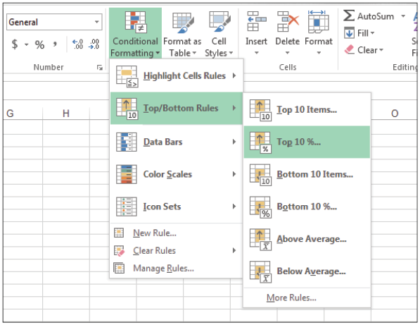
Instantly highlight important data with Conditional Formatting. - Click OK. Excel highlights the grades that fall within the Top 10%.
Removing conditional formatting in Excel
You can remove conditional formatting from an entire worksheet or a specified range following these steps:
- Select range A4:E37.
- Choose Conditional Formatting again.
- Choose Clear Rules.
- Select Clear Rules from Selected Cells.
Creating a new conditional formatting rule in Excel
If the predefined rules are not what you are looking for, you can create your own, including specifying the formatting you want to apply should the conditions be met. The next set of step shows you an example of how to use this feature.
- Select range E4:E37.
- From the Style group choose Conditional Formatting again.
- Choose New Rule.
- From the Rule list, select Format only cells that contain.
- In the Format only cells with sections, select Greater Than from the drop-down menu adjacent to the Cell Value field.
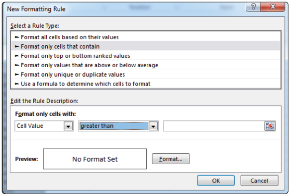
Create a New Rule to make your data standout when it meets specific criteria. - Type 2000 in the box adjacent to Greater Than.
- Click Format and choose the Fill tab.
- Select the color Blue.
- Click OK twice. Excel highlights all scores that are higher than 2000.