Excel Tutorial for beginners: Learning Excel Tools
This Excel tutorial for beginners explains the key Excel tools you need to know to work efficiently in Microsoft Excel. This tutorial is applicable to most versions of Microsoft Excel.
Excel Tools: Understanding the Excel Cursor Icon
Before we begin exploring the Excel workspace, it helps to get to know the mouse pointer as it takes many different forms in Excel. The pointer appears as the familiar arrow when you are choosing commands. When you move the mouse pointer within the worksheet area the mouse pointer changes its shape to that of a plus sign. As you enter data in a cell, the mouse pointer takes the shape of a cursor.
Since the mouse pointer takes so many different forms depending on the task you are performing it helps to take a moment to review the most basic shapes. The table below describes the mouse pointer shapes in more detail.
Excel cursor: mouse pointer shapes | |
Shape | Action |
| Choose a command |
| Select a cell |
| Enter or edit data in a cell |
| Extend a selection with the AutoFill handle |
| Resize columns and rows |
| Click to select the current row. |
| Click to select the current column. |


Understandign the Excel Ribbon
The Excel Ribbon, which runs along the top of the worksheet window, contains context-sensitive tools and commands to help you organize, calculate, and format your data. It is made up of a series of named tabs, each of which contains a set of related commands. For instance, the Home tab contains a set of frequently-used commands such as Copy and Paste. The names of the tabs are Home, Insert, Page Layout, Formulas, Data, Review, and View. Additional tabs are also displayed when working Charts, Images, and PivotTables.
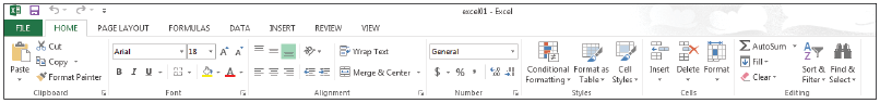
Excel Ribbon Commands.
The table below describes the options on the Excel Ribbon.
Tab | Description |
Home | Contains commonly used commands such as format cells, copy and paste, text alignment, and number formats. |
Insert | Commands that enable you to insert items into your worksheet including charts, images, text boxes, and SmartArt. |
Page Layout | Contains commands that enable you to change the appearance of your printed page. You can set margins, apply themes, change the page orientation, and insert page breaks |
Formulas | Contains function library and other commands related to performing calculations. |
Data | Contains commands for managing lists of data. |
Review | Contains commands such as Spell Checker, Grammar Checker, etc. |
View | Commands that enable you to change the display of the worksheet window. |
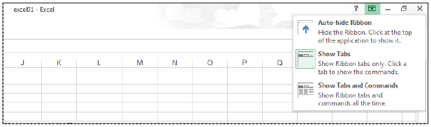
Customizing the Excel Ribbon display
You can collapse the Ribbon, by clicking the Ribbon Display Options button located in the far right corner of the title bar, so that only the named tabs appear across the top of the worksheet window. When you need to choose a command, just click the tab to redisplay the Ribbon and its options. You can also choose to Auto-Hide the Ribbon when you need additional viewing space. When you click the top of the worksheet window the Ribbon is redisplayed.
Collapse the Ribbon to display the named tabs only.
The table below describes the Ribbon Display Options found in the top-right corner of Excel.
Excel Option | Icon | What it Does in Excel |
Auto-Hide Ribbon | Hides the Ribbon. Click at the top of the Excel window to redisplay it. | |
Show Tabs | Display tabs only. Click a tab to redisplay the Ribbon. | |
Show Tabs and Commands |
| Displays both the Tabs and Commands at all times. |
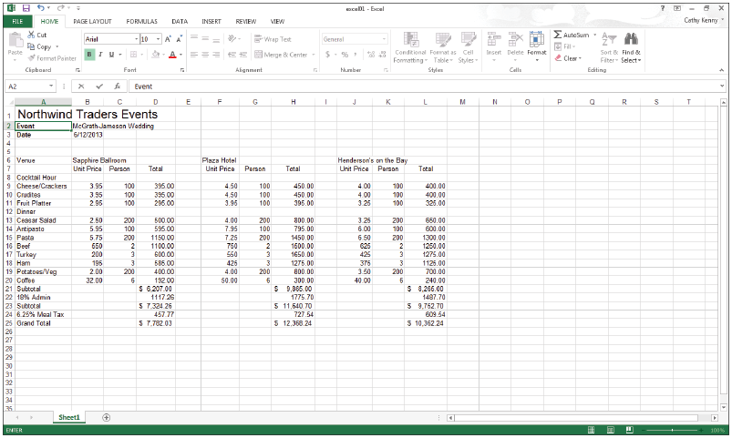
Collapsing the Ribbon in Excel
- Click the Ribbon Display Options button.
The Ribbon Display Options button allows you to alter the Ribbon’s appearance. - Choose Show Tabs and then select cell A
- Click the Home tab to redisplay the Ribbon and choose Bold in the Font group.
The Show Tabs command shows the tabs but doesn’t display the Ribbon unless a specific tab is selected. Once a command is selected on the Ribbon or you click elsewhere on the worksheet, the Ribbon disappears.
Hiding the Excel Ribbon
Use these steps to hide the Excel ribbon:
- Click the Ribbon Display Options button.
- Choose Auto-Hide Ribbon.
- Click the top of the Excel window to redisplay the Ribbon.
The Auto-Hide Ribbon command hides the Ribbon from view. When you click the top of the worksheet window, the Ribbon is redisplayed.
Once you choose a command or click elsewhere on the worksheet, the Ribbon disappears.
 | To quickly collapse the Ribbon, right-click anywhere within the Ribbon and choose Collapse the Ribbon. |
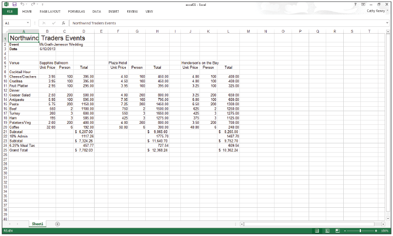
Exploring the Status Bar in Excel
The Status bar appears at the bottom of the worksheet window and provides updates on the current worksheet. Messages appear in the lower left corner to tell you what a command does, or what you should do next, to execute a command. For instance, when entering data in a cell the Status bar displays ENTER in the lower left corner.
The Status bar displays the word ENTER when entering data in a cell.
The Status bar also contains a set of buttons that enable you to change the view of your worksheet. You can switch between Normal, Page Layout, and Page Break Preview modes. Using the Zoom slider, you can enlarge or reduce the size of the worksheet display.
Switching display modes in Excel
The default viewing mode in Excel is the Normal mode, and it is primarily used when you are working with your data. There are times when you want to switch the display to see what your worksheet will look like when printed, or you may just want to view where the page breaks will occur, and you can use various display modes to see these things. You can quickly change the viewing mode of your worksheet by using the buttons in the Status bar. You’ll learn more about printing in Lesson 2, “Creating a Worksheet in Excel 2013.”
- Switch to Page Layout mode by clicking the Page Layout button.
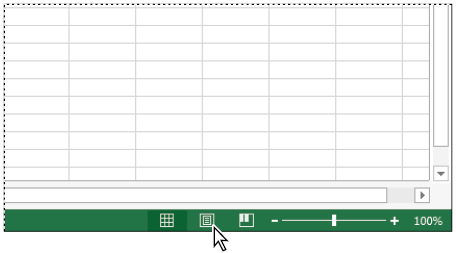
Choose the Page Layout mode. - Switch to Page Break Preview mode by clicking the Page Break Preview Button.
- Click Normal to return the regular viewing mode.
Change the magnification size of the worksheet display in Excel
You may need to change the size of your worksheet display, especially if you are working with data that extends beyond the visible area. Using the Zoom tool in the Status bar, you can quickly reduce or enlarge the worksheet display.
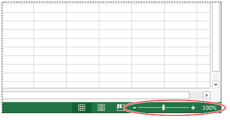
Change the size of your worksheet display by dragging the Zoom slider.
- Click and drag the Zoom slide to enlarge the display area to 125%.
- Drag the slider to 100% to return the view to its original size.
Customize the Quick Access Toolbar in Excel
The Quick Access Toolbar is displayed at the top left of the Excel window and provides single-click access to frequently-used commands such as Save and Undo. You can customize the toolbar to add additional commands that you use frequently by following these steps:
- Click the Customize Quick Access Toolbar button.
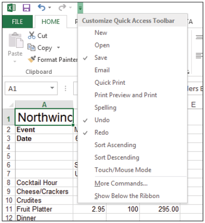
Add your favorite commands to the Quick Access Toolbar to gain single-click access. - Click New to add the New command to the toolbar.
- Click the Customize Quick Access Toolbar again and click Open to add the Open command to the toolbar.